Self-Balancing Reaction Wheel

Posted Feb 16, 2025 Updated Mar 24, 2025

By Austyn Loehr

29 min read

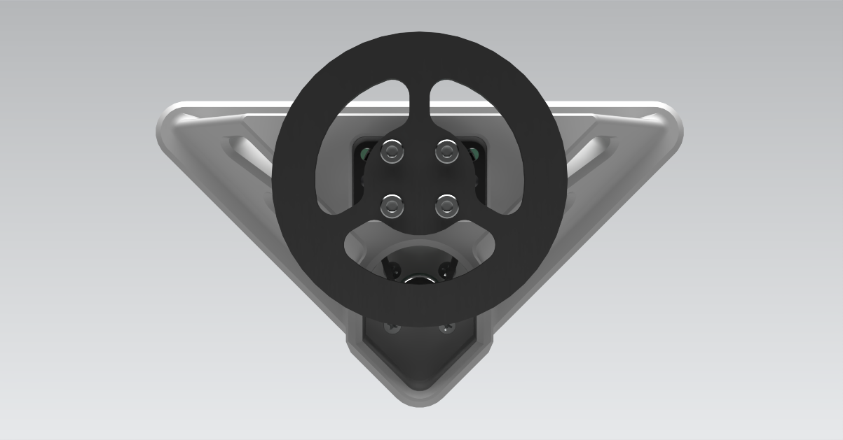
Demo

Overview

I started this project to expand my knowledge of embedded system design. I began learning embedded C in 2022 and wanted a project to practice and apply my skills. This project was inspired by The Cubli, though I chose to focus on balancing a single axis for my first project.

As a mechanical engineer, I have taken courses in control systems, and I saw this project as an excellent opportunity to apply some of that knowledge. While I have previously used Arduino in several college projects, I wanted to gain experience with a more industry-relevant microcontroller. I decided on the STM32 for its large support community and the extensive IDE.

In order to balance, this device relies on the conservation of angular momentum. The weighted flywheel is the key component of this design. As the flywheel’s speed changes, it generates a reaction torque that alters the orientation of the device. A brushless motor is coupled to the flywheel to control its speed. Similar reaction wheels are commonly used in spacecraft to control orientation.

All manufacturing files and source code for this project can be found in the GitHub repository here. Please note that, while this is a simple desk toy, the BOM cost is approximately $300. The biggest expenses are the PCB and the brushless motor controller. I approached this project as a hobby and learning experience, rather than prioritizing cost-effectiveness.

If you plan to recreate the device, I recommend using this project as a reference for your own design.

Mechanical Design

All of the 3D design work for this device was completed in NX. Although I purchased components such as the battery, motor, and pulleys, I designed and 3D printed many of the critical parts.

My first design challenge was sizing the motor and flywheel to create a device capable of jumping up and balancing on its own. To do this, I developed a Simulink model to simulate the system’s dynamics. Using rough estimates for weight and inertia, I calculated the minimum motor torque required for the reaction wheel to flip over. If the reaction wheel could flip from one side to the other, it would generate more than enough torque for effective balance control. The simulation model was super helpful because I was able to tweak different parameters and see how they affected the system.

PCB Design

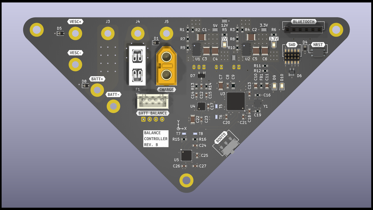Figure 1. Balance Controller Rendering

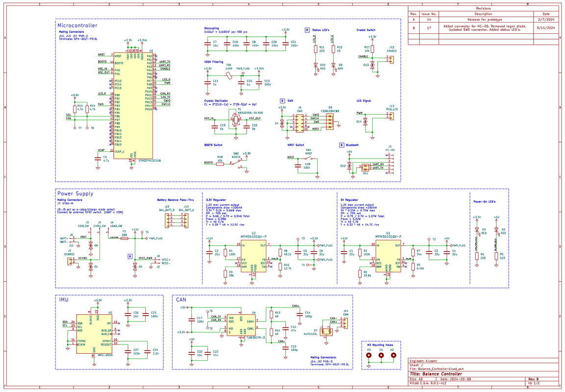Figure 2. Balance Controller Schematic (PDF)

Background

I was originally planning on having all the electronics housed on a breadboard, but as I got more into the project, I saw an opportunity to also learn PCB design with KiCad. Thanks to Phil’s Lab on YouTube, I was able to learn KiCad and the basics of designing a PCB for an STM32 MCU. His channel has a lot of great free content that covers many important aspects of PCB design, helping beginners get started with designing their own boards quickly. Before starting the design, I spent quite a bit of time doing my own research to ensure I understood critical design concepts. I wanted to make sure I was following best practices for signal integrity, such as proper component placement, selecting coupling capacitors, and managing return paths.

Design Requirements

Fits within designed chassis
12VDC input from battery
Export 12VDC, 20A (fused) to VESC motor controller
Provisions for emergency stop switch, cuts power to motor controller
STM32 MCU
MPU6050 IMU
Controllable status LEDs
CAN interface with 120 Ohm terminating resistor
UART interface

Power Supply

The board needed to export 12V and provide both 3.3V and 5V for onboard peripherals. Due to the 12V, 20A export requirement, much of the board was essentially a copper pour to handle this load. For handling the emergency stop, I decided to use a 3-position SPDT switch. This would allow all devices to be turned on or off and provide an additional circuit for charging. The idea for the charging circuit was to provide a means to charge the battery without powering any onboard devices.

For the 3.3V and 5V supplies, I chose to use two MPM3610GQV-P switched DC-DC converters. I selected these converters because they were able to handle a wide range of input voltages and met both my voltage and current output requirements. Each converter can output up to 1.2A, which is more than sufficient for my application. These converters were able to step down the 12V battery voltage to the 3.3V–5V range without generating significant heat. Configuring the output voltage for these converters was straightforward; it simply required designing the appropriate voltage divider circuit according to the datasheet.

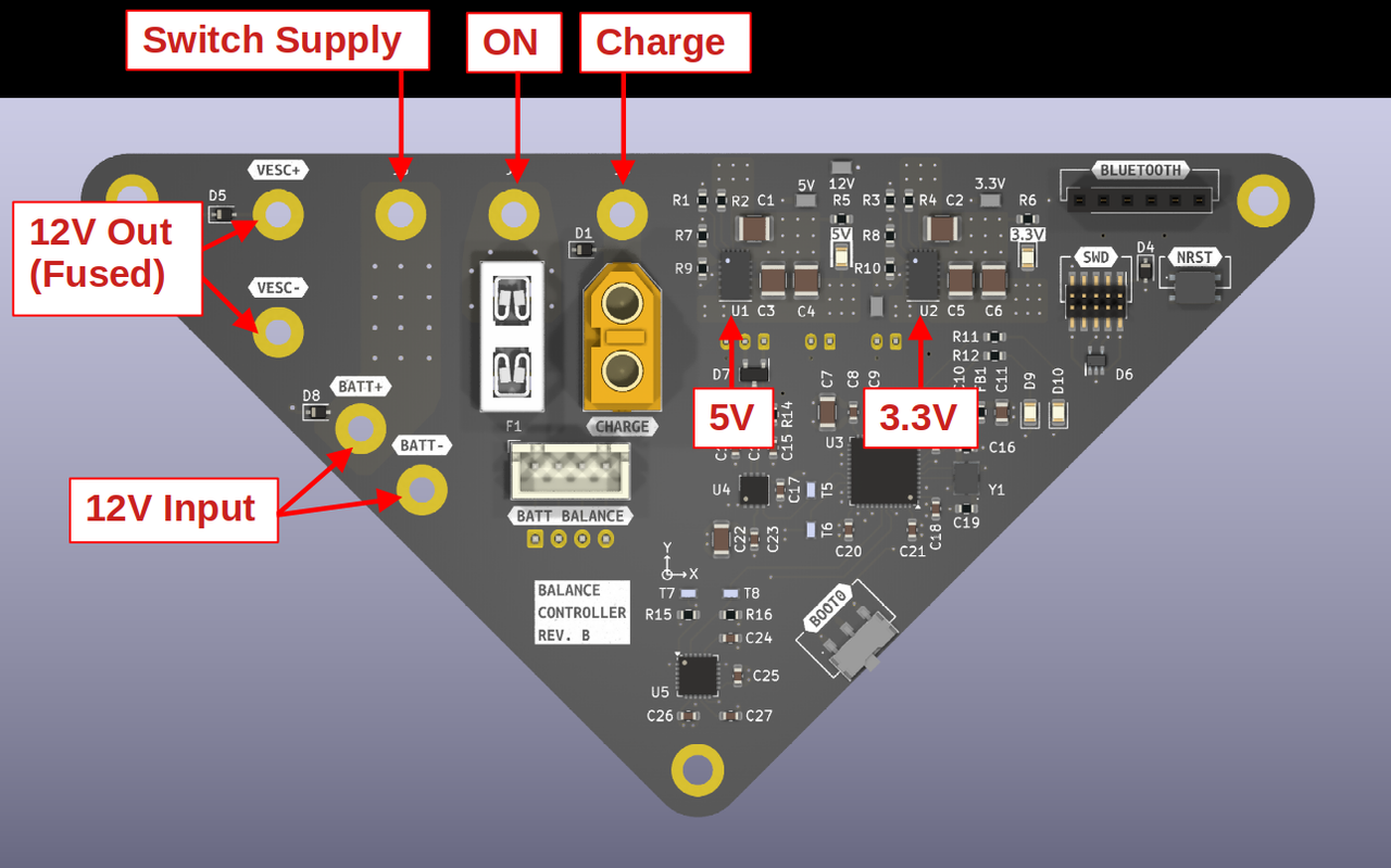Figure 3. Power Supply Overview

I chose to design a 4-layer PCB for this application. This allowed me to have one power supply layer, one ground layer, and two signal routing layers. The stack-up was as follows: signal 1, ground, power, signal 2. This design choice worked well for minimizing EMI and made routing power to all my components straightforward—all I had to do was drop a via to the power layer. Having a dedicated power layer gave me a lot of space on the first layer for signal routing, allowing me to fit 90% of the traces on it.

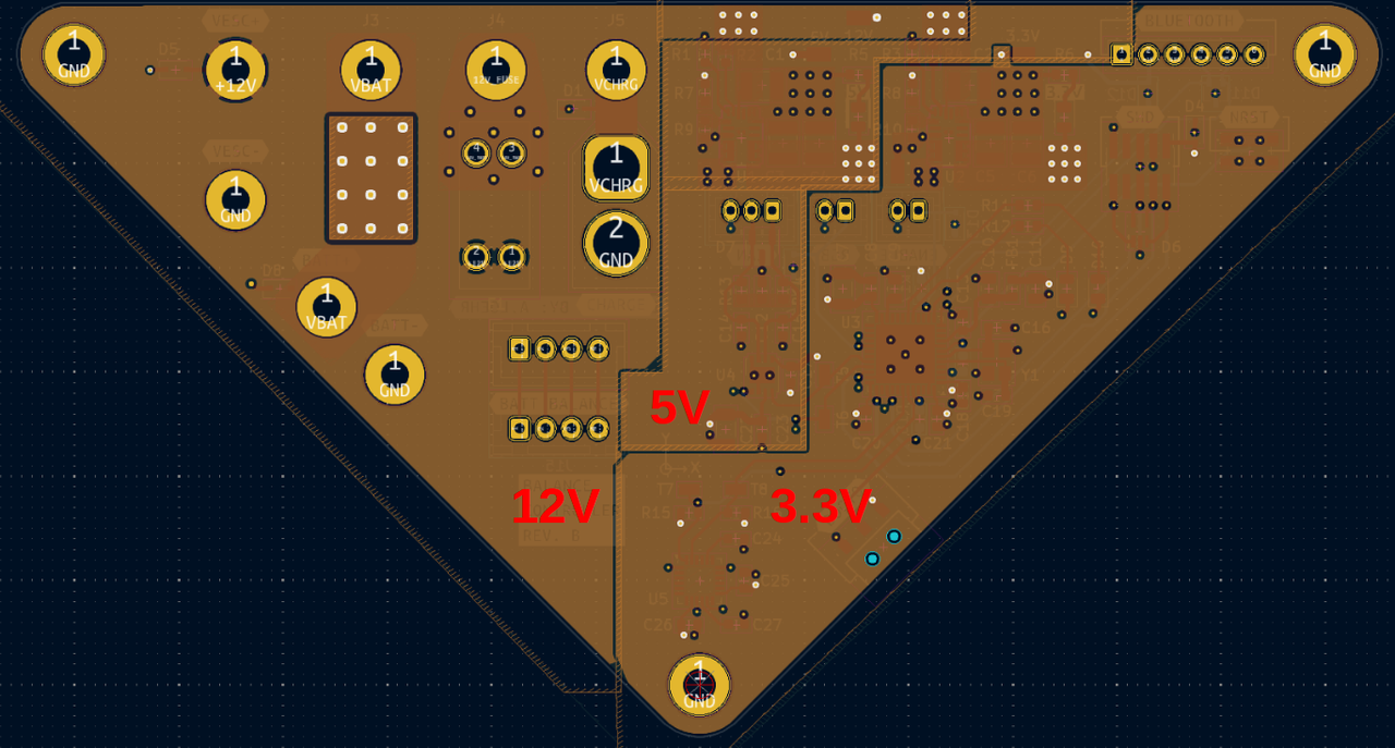Figure 4. Power Supply Layer

Component Integration

After the power supply strategy was figured out, selecting components for the board was fairly easy. Since this was my first PCB design, I was surprised at how straightforward it was to integrate the remaining ICs. Component datasheets contained all the necessary information to design any supporting circuits and select the proper resistors and decoupling capacitors.

The remainder of the board design was mainly a packaging exercise. Placing all the components in optimal positions while maintaining best practices for component spacing, trace width, and trace spacing was definitely the most time-consuming part of the design.

Areas For Improvement

The header labeled “Bluetooth” is designed to interface with an HC-05 as a plug-in Bluetooth module, though this was not my original intent. The first revision of the board actually had an RN4871, an onboard UART bluetooth module. Unfortunately, I was never able to get this module to work for my application. The goal was to log important signals over UART and wirelessly record the data on my computer. I spent a few weeks working with the configuration but was never able to maintain a connection longer than a few seconds on both Linux and Windows machines. The easiest solution was to integrate the HC-05 module. I did most of my initial testing with this device, and I knew it would work if I were to pay for a second board revision to be manufactured.

If my goal hadn’t been to learn how to program in the STM32 ecosystem, I would have replaced both the MCU and Bluetooth module with an ESP32 or a similar SOC that met my interface requirements. If I had gone in this direction, I think I would have used Wi-Fi with an IoT protocol instead of Bluetooth. I believe that would have made it much easier to interface with a computer and view live data. Maybe a project for another day…

The emergency stop circuit routes all battery current through a SPDT switch. It was difficult to find a switch in this form factor that was able to handle the 20A current requirement. If I were to revise the board, I would integrate two relays on the PCB and pass all current through them. The SPDT emergency stop switch would then just control the relay coils.

Oh and one last thing, the pinout on the charger connector is backwards from the normal convention. Never quite had the motivation to go back and fix that one.

Software Architecture

Top Level Architecture

To keep the software organized, I divided the program into four subsystems:

Configuration
Input/Output (IO)
Data Processing (PR)
Control (CT)

The configuration functions run once at startup, while the IO, PR, and CT functions execute sequentially in a super loop. This architecture keeps related functions grouped together and separates unrelated code, making the program easier to manage and maintain. This architecture is illustrated below in Figure 5.

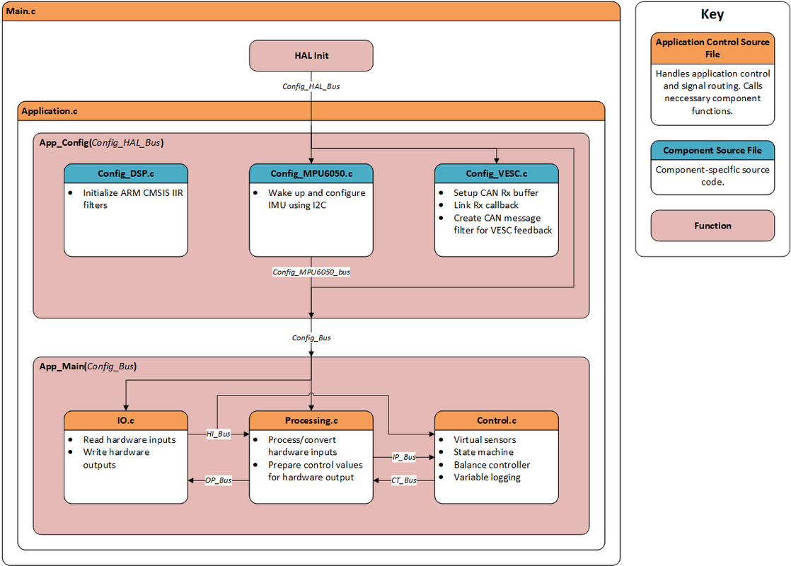Figure 5. Top Level Architecture

Data Bus Structure

Data is passed between different sections using structs. There are five top-level data buses that move data throughout the program:

Config Bus
Hardware Input Bus (HI)
Input Processing Bus (IP)
Control Bus (CT)
Output Processing Bus (OP)

Each top-level bus consists of smaller component buses. The HI_Bus struct below demonstrates how the HI bus is structured in this application. It is composed of sub-buses that are outputs from individual component IO libraries. This structure is beneficial because it simplifies data access and allows developers to easily trace the origin of each data signal. For example, it is immediately clear that HI_Bus.HI_VESC_Bus.MotorSpeed_rpm is a signal generated from the IO_VESC library.

  
typedef struct HI_Bus {
    HI_VESC_Bus_t HI_VESC_Bus;
    HI_MPU6050_Bus_t HI_MPU6050_Bus;
    HI_DiscreteInput_Bus_t HI_DiscreteInput_Bus;
} HI_Bus_t;

typedef struct HI_VESC_Bus {
    int32_t MotorSpeed_rpm;
    int32_t MotorCurrent_mA;
} HI_VESC_Bus_t;

Subsystem Architecture

Figures 6–8 illustrate how the IO, PR, and CT systems are structured and how data flows between their components.

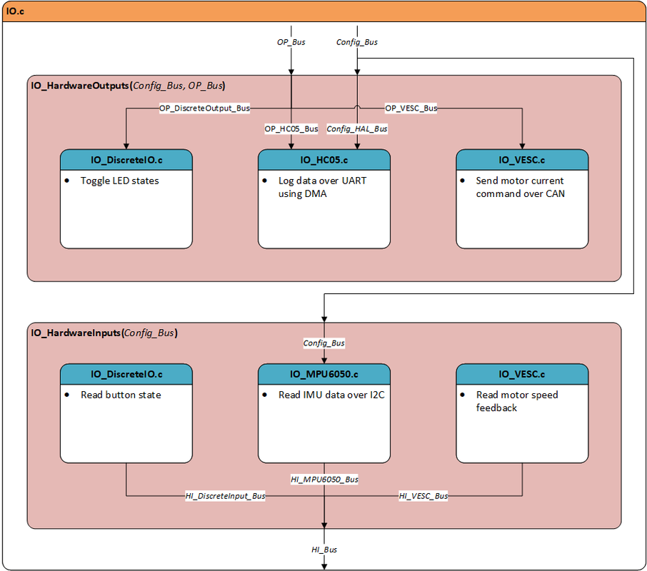Figure 6. Input/Output Subsystem Architecture

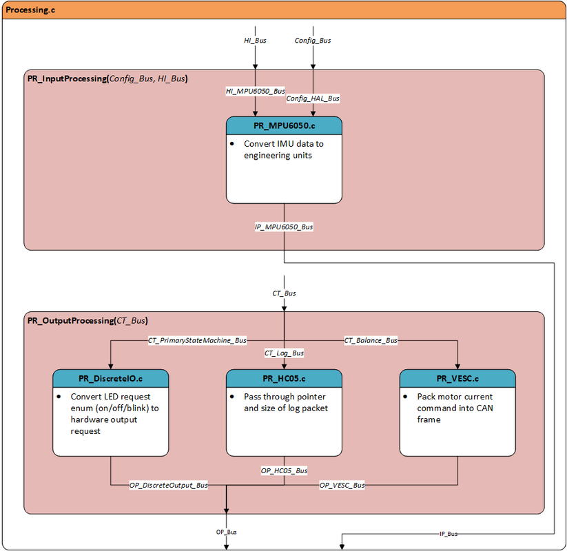Figure 7. Data Processing Subsystem Architecture

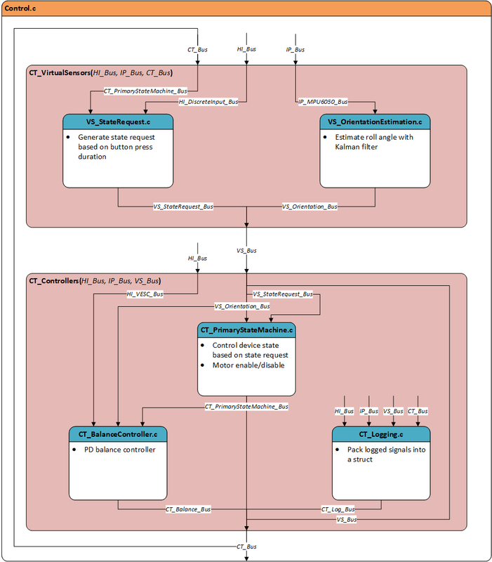Figure 8. Control Subsystem Architecture

State Machine

Two state machines control the state of the reaction wheel: State Request and Primary State Machine. To shorten development time, these state machines were designed using Simulink Stateflow, and C code was autogenerated.

State Request

Figure 9 illustrates the State Request state machine. The user can request one of three possible states:

Standby: Stop balancing
Balance: Start balancing
CalibrateIMU: Calibrate IMU

The user can transition between Standby and Balance by pressing the control button for 200ms. To calibrate the IMU, the device must be in Standby, and the button must be held for 5 seconds.

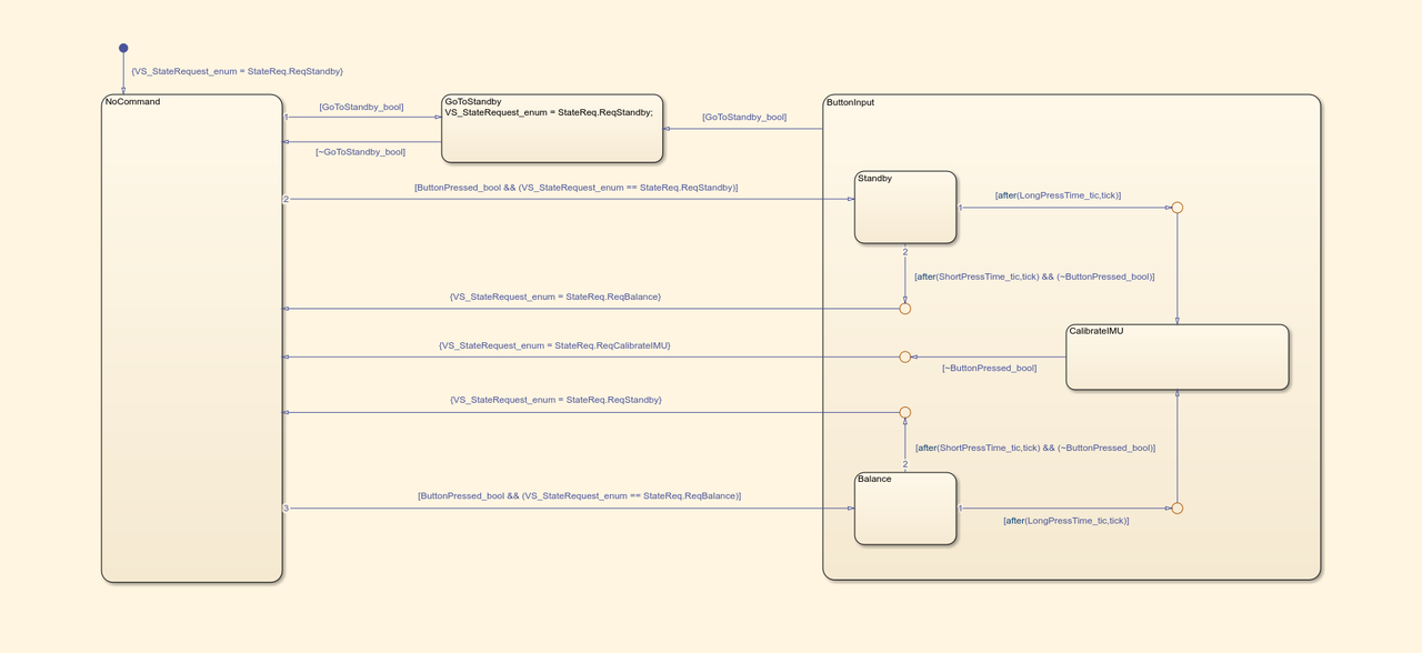Figure 9. State Request Diagram

Primary State Machine

Figure 10 illustrates the Primary State Machine. The device can operate in one of four main states:

Error: Motor disabled, error interupt triggered
Standby: Motor disabled, stops balancing
MotorEnabled: Motor enabled, begins balancing
CalibrateIMU: Motor disabled, initiates IMU calibration process

When in the MotorEnabled state, the device can be in one of two substates:

JumpUp: Roll angle over $30^\circ$, initiates jump up procedure
Balance: Roll angle under $20^\circ$, PD controller maintains balance

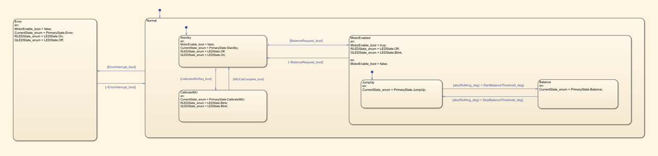Figure 10. Primary State Machine Diagram

Angle Estimation

To design a balance control system, I first needed accurate feedback of the device’s current angle. The balance controller PCB includes an onboard IMU (MPU-6050) with both an accelerometer and a gyro. I used data from these sensors to estimate the reaction wheel’s orientation.

Accelerometer Estimate

Using the accelerometer, I was able to calculate the current angle using the gravity vector. Since the device only rotates around a single axis, the angle can be estimated using only the X and Y acceleration measurements. If the device is perfectly balanced and unaffected by external forces, the gravity vector would align with the IMU’s Y-axis, and $a_y$ would read around 9.8 m/s². As the device deviates from this position, more of the gravity vector will be in the IMU’s X-axis, and the magnitude of $a_x$ would increase while $a_y$ decreases. Using basic trigonometry, the device’s angle can be estimated using equation \eqref{eq:theta_accel}.

\[\begin{equation} \theta = \tan^{-1}\left(\frac{a_x}{a_y}\right) \label{eq:theta_accel} \end{equation}\]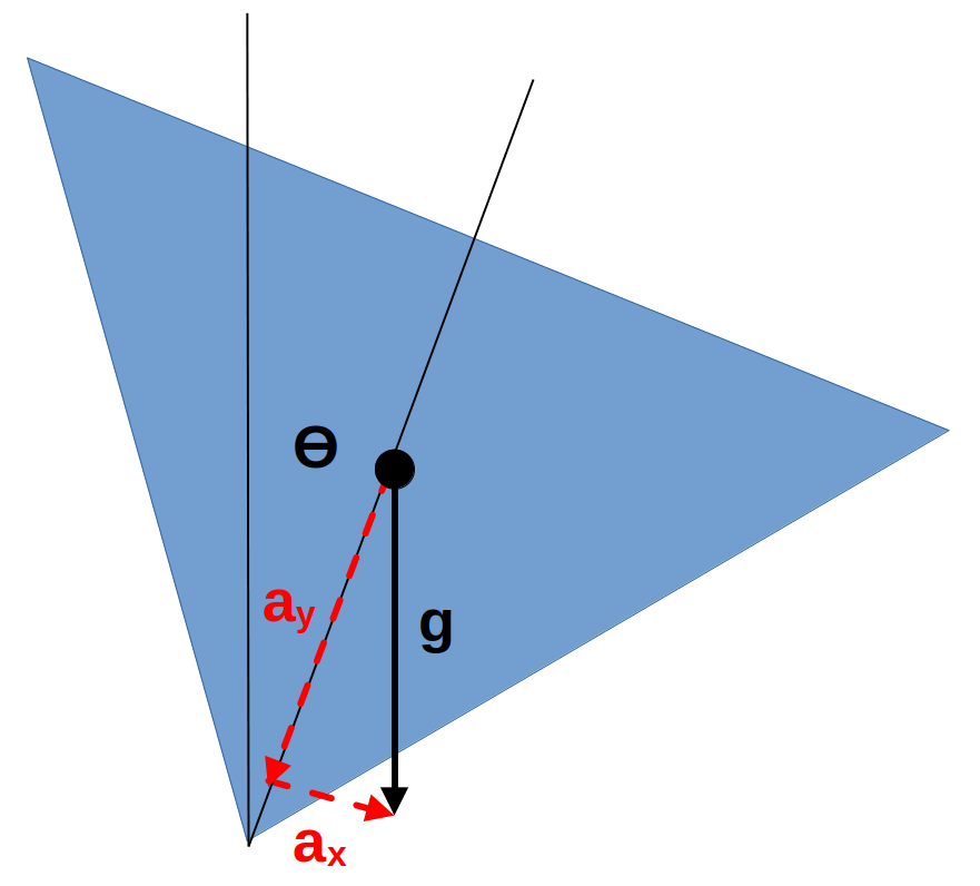

Figure 11. Accelerometer Angle Calculation

This estimate is only accurate if there are no external net-forces, other than gravity, acting on the system. Any other net-forces will be seen in the accelerometer measurements, and throw off the angle estimate. This estimate is only accurate if there are no external net forces, other than gravity, acting on the system. Any other net forces will be detected by the accelerometer and will throw off the angle estimate. The advantage of this method is that it can always calculate an estimate of the device’s orientation without needing information about its previous position.

Gyro Estimate

Using the gyro, I was able to calculate the current angle by integrating the device’s angular velocity from a known starting position. Assume the device is rotating at a constant 1000 deg/s and the initial angle of the device is known to be 45 degrees. If the device rotates for 5 ms, it will have rotated a total of 5 degrees, ending at a new angle of 50 degrees. This same concept applies, except that the angular velocity is not constant. This is not a problem, since the gyro can measure the device’s angular velocity ($\omega$) at any point in time. This concept is described by equation \eqref{eq:theta_gyro}.

\[\begin{equation} \theta = \int_{t_0}^{t} \omega(t) \, dt \label{eq:theta_gyro} \end{equation}\]

Unfortunately, this continuous system cannot be perfectly modeled on an embedded system. However, it can be approximated using Euler’s method for integration, as shown in equation \eqref{eq:theta_gyro_euler}. In this method, the current angular velocity is multiplied by the sample time to calculate an angular displacement, which is then added to the previous angle to obtain the current angle. While there are more accurate methods for discrete integration, this approach proved sufficient for my application. The estimation algorithm ran at 500 Hz, which helped minimize integration errors.

\[\begin{equation} \theta_{n} = \theta_{n-1} + \Delta t \cdot \omega_n \label{eq:theta_gyro_euler} \end{equation}\]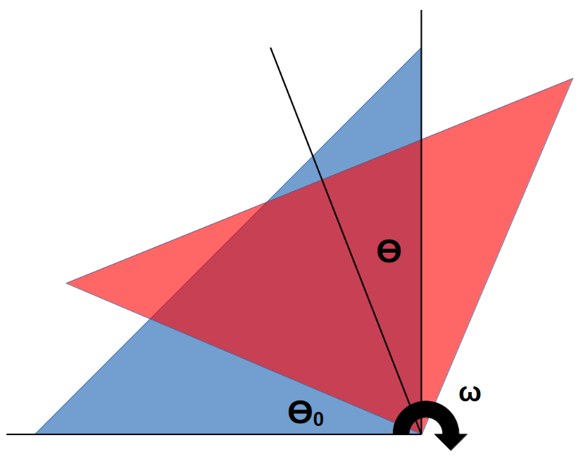

Figure 12. Gyro Angle Calculation

The main advantage of this estimation method is that it is less susceptible to external forces. However, there are some drawbacks: you must know the device’s initial position, and the estimate will gradually drift over time. This drift occurs because sensor noise accumulates as it is integrated over time.

Comparison

The following plots show real data that was logged from the reaction wheel’s IMU. The motor was spinning at a constant speed of approximately 5500RPM. The reaction wheel was manually flipped from one side (+45 degrees) to the other (-45 degrees). At $t=16s$, the reaction wheel motor was turned off to compare sensor noise. Data from the IMU was logged via bluetooth with a sample rate of 500Hz. Equations \eqref{eq:theta_accel} and \eqref{eq:theta_gyro_euler} were implimented in Python on my desktop. All angle estimation calculations and filtering were performed during post-processing.

Figure 13 shows the results of passing raw $a_x$ and $a_y$ values into equation \eqref{eq:theta_accel} to estimate the reaction wheel’s orientation. Lines are drawn at $y = \pm 45^ \circ$ for reference, marking the true positions of the reaction wheel when flipped on its side. Note the drastic difference in noise when the motor is turned on versus off. This noise is the result of vibrations that are generated from the motor and propogated through the whole system. I attempted to mitigate this issue by mounting the balance controller PCB on rubber isolators, but unfortunately, they were unable to provide sufficient damping. While trends in the data are visible, the measurements are essentially unusable with the motor running. However, the estimates appear to be accurate when the motor is turned off.

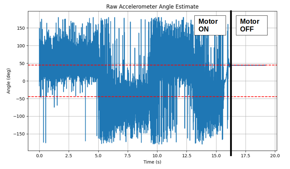Figure 13. Raw Accelerometer Angle Estimate

Figure 14 shows the same data but $a_x$ and $a_y$ values were each passed through a 1st order digital low-pass filter (butterworth) before being passed into equation \eqref{eq:theta_accel}. Cutoff frequencies of 20Hz, 5Hz, and 1Hz are compared. Each of these filtered examples represents a significant improvement over the raw data in Figure 7. Both the 20 Hz and 5 Hz filters still exhibit considerable steady-state noise and large angle spikes when the device falls on its side. Based on this data, the 1 Hz filter appears promising—at least for now.

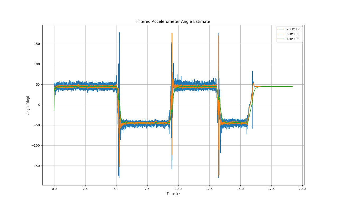Figure 14. Accelerometer Filter Comparison

Figure 15 contains the same data as Figure 14, but zoomed in on the timeframe $t=[15s, 17s]$. This figure highlights the biggest disadvantage of additional filtering: response time. While the 1 Hz filter exhibits significantly less noise, it takes much longer to respond to changes in position. This increased response time is not acceptable for this application.

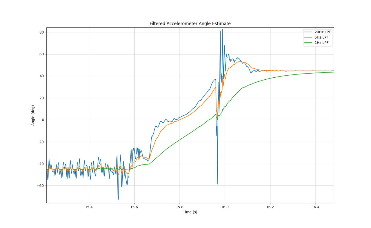Figure 15. Filter Response Time Comparison

Figure 16 shows the results of passing $\omega_z$ into equation \eqref{eq:theta_gyro_euler} with an initial condition of $45^ \circ$. Note that no additional filtering was performed on this data, and the signal is already much smoother compared to the accelerometer data. While the estimate initially starts off accurate, you can see it begin to drift around $t=10$ . Unfortunately, this drift is also not acceptable for this application.

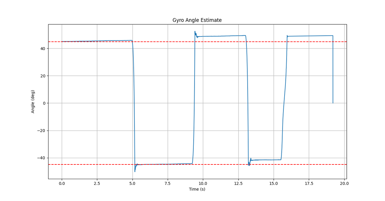Figure 16. Gyro Angle Estimate

Figure 17 shows a comparison between gyro and filtered accelerometer angle estimates. If only there were a way to somehow combine these two estimates into a single, more accurate estimate…

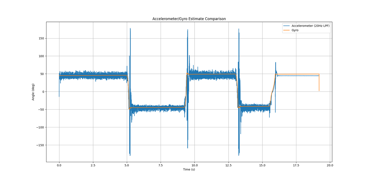Figure 17. Accelerometer/Gyro Comparison

Kalman Filter

I’d like to preface this section by mentioning that the Kalman filter was not my first choice for the orientation estimation in this project. In fact, I initially tried to avoid designing a Kalman filter. I first explored using only the gyro with some integrator reset conditions, as well as a complementary filter. I initially achieved good results with the complementary filter, until I assembled the first prototype. The vibrations induced by the motor rendered both of these strategies unusable. This forced the project to be put on hold for several weeks while I learned about Kalman filter design.

For anyone looking to learn about the topic without wading through formal proofs and intimidating matrix math, Kalman and Bayesian Filters in Python is a fantastic resource. The author does an amazing job of breaking down concepts into layman’s terms and providing real examples of how to implement the filters in Python.

I don’t intend on explaining the low-level matrix math behind this filter, but I will cover the design decisions that went into picking the input matrices.

Equations of Motion

I had the choice of using a constant velocity (first-order) or constant acceleration (second-order) model for this application. While designing the filter, I was able to achieve much better results with the second-order model, so I decided to go with this approach. To begin designing the state-space model for the reaction wheel, I started with Newton’s fundamental equations of motion for an object undergoing constant acceleration (equations \eqref{eq:newton_pos} - \eqref{eq:newton_accel}).

\[\begin{equation} \theta = \theta_{0} + \dot{\theta} \Delta t + \frac{1}{2} \ddot{\theta} \Delta t^2 \label{eq:newton_pos} \end{equation}\] \[\begin{equation} \dot{\theta} = \dot{\theta}_0 + \ddot{\theta} \Delta t \label{eq:newton_vel} \end{equation}\] \[\begin{equation} \ddot{\theta} = \ddot{\theta} \label{eq:newton_accel} \end{equation}\]

State Matrix

To convert equations \eqref{eq:newton_pos} - \eqref{eq:newton_accel} to state space representation, they need to be expressed in matrix form, following the format shown in equation \eqref{eq:state_space_control}. The term $\mathbf{B} \mathbf{u}$ represents any control inputs to the system. This term would be used if I wanted to include the commanded motor speeds in the model to further improve my estimate. My goal was to keep the model as simple as possible to achieve acceptable estimate accuracy. I found that I was able to get adequate results without including these inputs. Therefore, equations \eqref{eq:newton_pos} - \eqref{eq:newton_accel} need to be converted to the form shown in equation \eqref{eq:state_space_nocontrol}. The state space model used for this filter is shown in equation \eqref{eq:state_space_model}.

\[\begin{equation} \mathbf{\bar x} = \mathbf{F} \mathbf{x} + \mathbf{B} \mathbf{u} \label{eq:state_space_control} \end{equation}\] \[\begin{equation} \mathbf{\bar x} = \mathbf{F} \mathbf{x} \label{eq:state_space_nocontrol} \end{equation}\] \[\begin{equation} \mathbf{\bar x} = \begin{bmatrix} \theta \\ \dot{\theta} \\ \ddot{\theta} \end{bmatrix} = \begin{bmatrix} 1 & \Delta t & \frac{1}{2} \Delta t^2 \\ 0 & 1 & \Delta t \\ 0 & 0 & 1 \end{bmatrix} \begin{bmatrix} \theta \\ \dot{\theta} \\ \ddot{\theta} \end{bmatrix} \label{eq:state_space_model} \end{equation}\]

Process Noise Matrix

The repository I mentioned above provides a great explanation of this process noise model (link). The model essentially assumes that acceleration is constant for the duration of each time period but may differ across time periods. One advantage of this approach is that you can model noise using a single $\sigma_x ^ 2$ value. In layman’s terms, this represents the expected amount of error in the model for each time period. This matrix can be tweaked to prioritize model estimates over measurements, or vice versa. The value for $\sigma_x$ was developed through testing.

\[\begin{equation} \mathbf{Q} = \begin{bmatrix} \frac{\Delta t ^ 4}{4} & \frac{\Delta t ^ 3}{2} & \frac{\Delta t ^ 2}{2} \\ \frac{\Delta t ^ 3}{2} & \Delta t ^ 2 & \Delta t \\ \frac{\Delta t ^ 2}{2} & \Delta t & 1 \end{bmatrix} \sigma_x ^ 2 \end{equation}\] \[\begin{equation} \sigma_x = 10 \end{equation}\]

Measurement Matrix

This filter takes two measurement inputs: $\theta$ and $\dot{\theta}$. Accelerometer measurements, $a_x$ and $a_y$, are each passed through a second-order, 20 Hz low-pass filter before being input into equation \eqref{eq:theta_accel} to calculate an estimated angle. This angle estimate is then fed into the filter as $\theta$. Raw gyro measurements are directly passed into $\dot{\theta}$. The measurement matrix used for this filter is shown in equation \eqref{eq:measurement_matrix}.

\[\begin{equation} \mathbf{z} = \begin{bmatrix} \theta \\ \dot{\theta} \end{bmatrix} \label{eq:measurement_matrix} \end{equation}\]

Next, a measurement function matrix needs to be designed to convert a state ($\mathbf{\bar x}$) into a measurement ($\mathbf{z}$). This conversion is described in equation \eqref{eq:measurement_form}. The measurement function ($\mathbf{H}$) for this filter is shown in \eqref{eq:measurement_func}.

\[\begin{equation} \mathbf{z} = \mathbf{H} \mathbf{x} \label{eq:measurement_form} \end{equation}\] \[\begin{equation} \mathbf{z} = \begin{bmatrix} \theta \\ \dot{\theta} \end{bmatrix} = \begin{bmatrix} 1 & 0 & 0 \\ 0 & 1 & 0 \end{bmatrix} \begin{bmatrix} \theta \\ \dot{\theta} \\ \ddot{\theta} \end{bmatrix} \label{eq:measurement_func} \end{equation}\]

Measurement Noise Matrix

The measurement noise matrix describes how much error is present in each of the measurements. The accelerometer will have some steady-state error due to vibrations and large spikes due to impacts. The gyro measurements only seem to be incorrect during an impact. This matrix can be tweaked to prioritize one measurement over another. The values below were developed through testing and resulted in adequate accuracy for this application.

\[\begin{equation} \mathbf{R} = \begin{bmatrix} \sigma_{\theta} ^ 2 & 0 \\ 0 & \sigma_{\dot{\theta}} ^ 2 \end{bmatrix}= \begin{bmatrix} 8 ^ 2 & 0 \\ 0 & 8 ^ 2 \end{bmatrix} \label{eq:measurement_noise} \end{equation}\]

Initial Conditions

The final step in designing the filter is determining the model’s initial conditions. The selection of these values affects the filter’s initialization performance. Initialization time is not critical for this application. As long as the filter converges to an accurate orientation estimate within a few seconds, that is sufficient. The initial position of the reaction wheel can range between $\pm 45^\circ$, though it is likely to start at either $+45^\circ$ or $-45^\circ$. To keep initialization simple, I set the initial angle estimate to $0^\circ$, as represented by $\mathbf{X}[0]$ in the model. The model also assumes that the device starts from rest and is not accelerating, as shown by $\mathbf{X}[1]$ and $\mathbf{X}[2]$. The initial model state is represented by equation \eqref{eq:x_initial}.

\[\begin{equation} \mathbf{X} = \begin{bmatrix} \theta \\ \dot{\theta} \\ \ddot{\theta} \end{bmatrix} = \begin{bmatrix} 0 \\ 0 \\ 0 \end{bmatrix} \label{eq:x_initial} \end{equation}\]

The confidence in the initial state can be specified using the initial covariance matrix \eqref{eq:p_initial}. Although the exact initial position of the device is unknown, we know it lies within the range of $\pm 45^\circ$, and this uncertainty is captured by $\mathbf{P}[0]$. To avoid overconfidence in the initial velocity and acceleration estimates, $\mathbf{P}[1]$ and $\mathbf{P}[2]$ are set to non-zero values. This approach helps the filter converge more quickly to an accurate orientation estimate.

\[\begin{equation} \mathbf{P} = \begin{bmatrix} \sigma_{\theta} ^ 2 & 0 & 0 \\ 0 & \sigma_{\dot{\theta}} ^ 2 & 0 \\ 0 & 0 & \sigma_{\ddot{\theta}} ^ 2 \end{bmatrix} = \begin{bmatrix} 45 ^ 2 & 0 & 0 \\ 0 & 4 ^ 2 & 0 \\ 0 & 0 & 4 ^ 2 \end{bmatrix} \label{eq:p_initial} \end{equation}\]

Filter Performance

While designing the filter, I found it easiest to first simulate it using logged data from the IMU in Python with FilterPy. This approach allowed me to focus solely on tuning the filter inputs, without having to worry about the correctness of my matrix math or embedded implementation. The library made it very easy to implement a Kalman filter and begin tuning. It also offers the capability to implement non-linear Kalman filters.

Figures 18 and 19 below compare the performance of the Kalman filter with that of accelerometer and gyro estimation methods, using the same data as Figures 15-18. In Figure 18, you can see that the filter initially tracks very closely to the gyro estimate. While the gyro estimate begins to drift over time, the filter maintains an accurate estimate. Additionally, note how much smoother the signal is compared to the accelerometer estimate. This demonstrates that the filter can effectively incorporate the accelerometer data without introducing any noise from the motor vibrations.

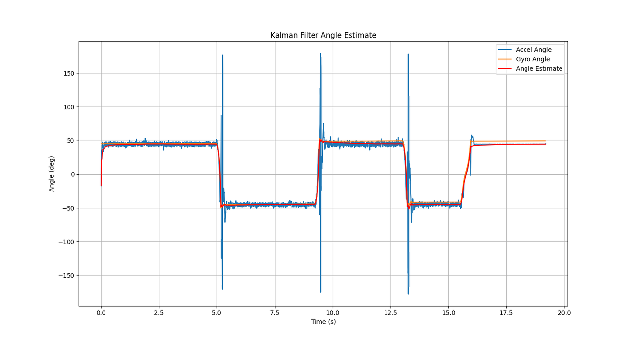Figure 18. Simulated Kalman Filter Overview

The drift in the gyro estimate is much more evident in Figure 19, where you can see how the estimate deviates from $45^\circ$ when the reaction wheel is on its side. Meanwhile, the filter tracks the mean accelerometer estimate with minimal noise. The estimate is even smoother than the 1Hz filtered accelerometer estimate shown in Figure 16, with almost no time delay!

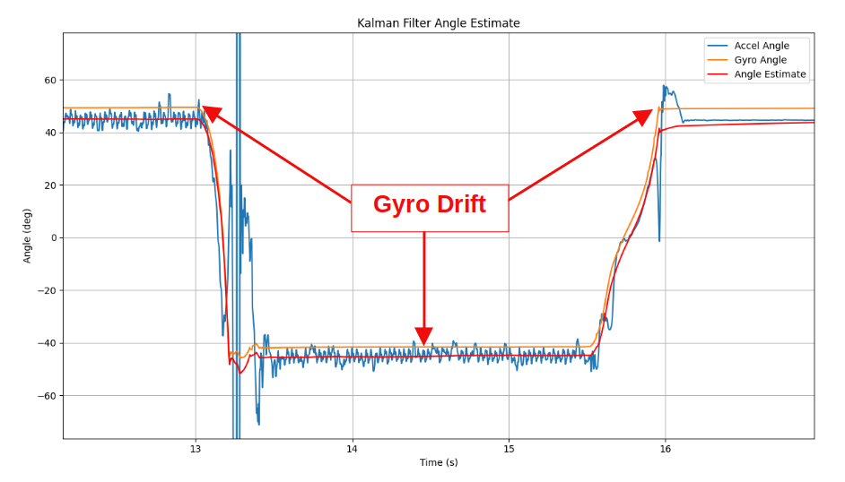Figure 19. Simulated Kalman Filter Comparison

Once I was satisfied with the simulated filter performance, the next step was to implement it in C on the MCU. To handle the digital filtering and matrix math, I utilized ARM CMSIS. While I won’t go into the details of the C implementation, but the source code for the filter can be found here.

Figures 20 and 21 below show actual Kalman filter data logged from the MCU. Figure 20 compares the filter with the gyro and accelerometer estimates. Performance of the real-time filter seems to align well with the simulation results.

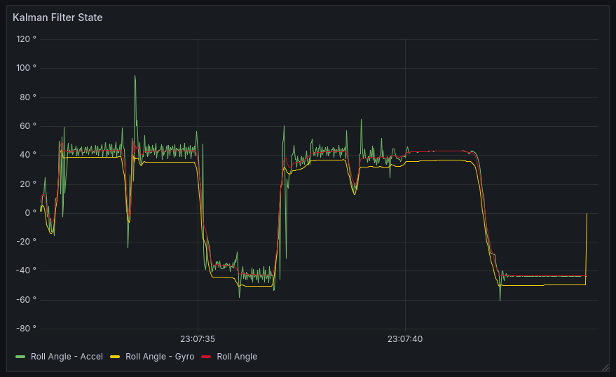Figure 20. Kalman Filter Real-Time Performance

Finally, the real-time initialization performance is shown in Figure 21 below. As you can see, the filter takes about 1 second to converge on an accurate orientation estimate. This initialization time is more than acceptable for the application.

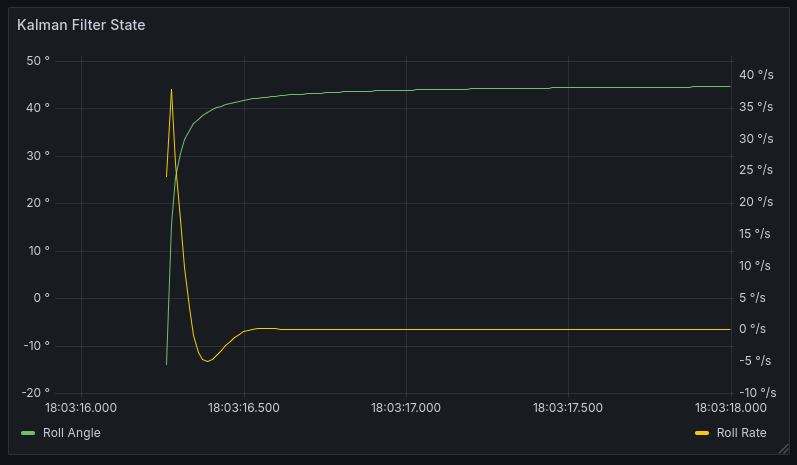Figure 21. Real-Time Initialization

Balance Control

Once I was able to calculate a robust orientation estimate, I was able to design the balance controller. The balance controller has two possible states: JumpUp and Balance.

Jump Up

The goal of this mode was to force the reaction wheel to jump as close to the center as possible without excessive overshoot. This is achieved by spinning the motor in one direction and then quickly reversing it. The reaction wheel spins up to 4100 RPM for 60 ms before rapidly switching the speed command to -4100 RPM. The sign of the speed command depends on which side the reaction wheel is currently on. The device will enter this mode when the current angle is greater that $30 ^ \circ$ and will exit when the angle is less than $20 ^ \circ$. It will continually attempt to jump to center until balanced or user requests Standby.

In this state, the motor controller operates in speed control mode. This means that the MCU sends a speed request to the motor controller, which is responsible for generating the current commands to control the motor speed.

I attempted the same strategy using current control mode but found that the device was significantly less responsive. It appeared that the motor controller applied a current rate limit to the command, causing the torque to slowly ramp down from driving torque to zero torque before applying regen torque. Whereas in speed control mode, the motor could immediately switch from driving torque to regen torque and target the requested speed.

Balance

Once the device exits the JumpUp state, it will enter the Balance state. In this state, a PD controller is used to maintain balance and a proportional controller is used to limit motor speed.

Since the reaction wheel relies on changes in speed to alter orientation, it is considered saturated when its max speed is reached. When using just a PD controller, I found that the device was only able to balance for a brief period of time before reaching max speed and falling on its side. As a result, the second controller was added to prevent saturation. Figure 22 below shows the block diagram for this control strategy.

In this state, the motor controller operates in current control mode, which provided smoother motor control at low speeds. As the device approaches $0 ^ \circ$, the motor torque gradually ramps down to zero. In speed control mode, the motor controller would apply a significant amount of regen torque to target zero speed, this would disrupt the balance of the device.

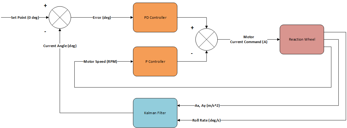Figure 22. Balance Controller Block Diagram

Performace

Figures 23 and 24 below show the reaction wheel’s balance performance with the final controller gains. The reaction wheel was able to jump up and balance in under 1.5 seconds, with approximately $10 ^ \circ$ of overshoot. It is also able to effectifly reject any disturbances, although there is quite a bit of overshoot in this scenario. While better performance could be achieved with additional tuning time or more advanced control strategies, I am very satisfied with this performance given the simplicity of the control algorithm.

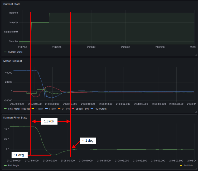Figure 23. Jump Up Response

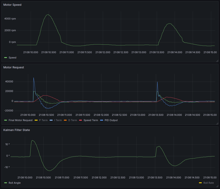Figure 24. Disturbance Rejection

Data Logging & Visualization

The final requirement for this device was the ability to wirelessly log and view data from the MCU. While I can view live data using STM32’s debugger, it lacks a user-friendly interface for logging and plotting data. I frequently used the debugger during the initial firmware development, but for tuning, I wanted an intuitive interface for plotting and comparing signals. The wireless data logging architecture is shown below in Figure 25.

Figure 25. Data Logging Architecture

Wireless Data Transfer

All logged data is sent over Bluetooth using the HC-05 UART Bluetooth module. This device handles all Bluetooth communication and requires data to be sent to it via UART, making integration with the STM32 very straightforward. In the MCU, all logged signals are packed into a struct and sent over UART in the following format:

  
typedef struct LogPayload{
    uint32_t tick_ms;
    float ax_mps2;
    float ay_mps2;
    float wz_dps;
    float axFilt_mps2;
    float ayFilt_mps2;
    float rollAngle_deg;
    float rollRate_deg;
    int32_t MotorSpeed_rpm;
    int32_t MotorCurrent_mA;
    int32_t MotorRequest_na;
    int32_t PIDTerm_mA;
    int32_t MotorSpeedTerm_mA;
    int32_t pTerm_mA;
    int32_t iTerm_mA;
    int32_t dTerm_mA;
    uint8_t MotorControlMode_enum;
    uint8_t StateReq_enum;
    uint8_t CurrentState_enum;
    uint8_t MotorEnable_bool;
} __attribute__ ((packed)) LogPayload_t;

Any connected bluetooth device is able to receive and unpack this struct for processing. Tick represents the timestamp at which the struct was packed. This log data packet is sent from the reaction wheel every 14ms. I was not able to run the data logger at the base execution rate of 500Hz, due to data throughput limits at 460800 baud. If I wanted to log data faster I could’ve sacrificed signal resolution and packed the data into fewer variables, but this was easy and worked fine for my application.

Logging and Visualization

Since the reaction wheel only broadcasts data, a host computer is required to log it. Once the Bluetooth connection is established, I use Minicom to receive the data and log the raw hex values to a file. Using Python, the hex data is read from the log file, unpacked into signals, and stored in an InfluxDB database. I chose InfluxDB because it is designed for time-series data, has an easy-to-use Python API, and integrates seamlessly with Grafana. Once the data is stored in the database, it can be easily viewed in Grafana. Grafana is a visualization platform that allows users to easily create dashboards for analyzing data. This made it easy to compare data from different tests while tuning the device, saving a significant amount of time compared to manually plotting and analyzing datasets with Python. The Grafana dashboard I created for this project is shown below in Figure 26.

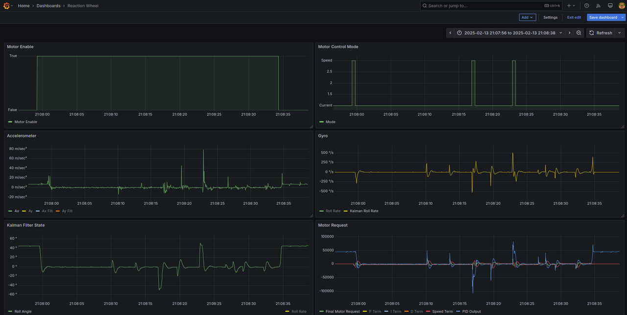Figure 26. Grafana Dashboard

Final Remarks

Overall, this project provided valuable insights into embedded system design. From PCB design to firmware development, each step presented unique challenges that helped me expand my knowledge and skill set. I improved my PCB design skills and gained a deeper understanding of microcontrollers, embedded software architecture, digital filtering, Kalman filtering, and control theory. While there is always room for improvement—such as refining the control algorithms or improving PCB design—the current implementation serves as a solid foundation for future enhancements. I hope this write-up helps others working on similar projects, and I look forward to applying my new skills to future projects.